4.2.44. POLY_ANISO
The POLY_ANISO program is a routine which allows a semi-ab initio description of the (low-lying) electronic structure and magnetic properties of polynuclear compounds. It is based on the localized nature of the magnetic orbitals (i.e. the d or f orbitals containing unpaired electrons [110, 111]). For many compounds of interest, the localized character of magnetic orbitals leads to very weak character of the interactions between magnetic centers. Due to this weakness of the interaction, the metals’ orbitals and corresponding localized ground and excited states may be optimized in the absence of the magnetic interaction at all. For this purpose, various fragmentation models may be applied. The most commonly used fragmentation model is exemplified in Figure 4.2.44.1.
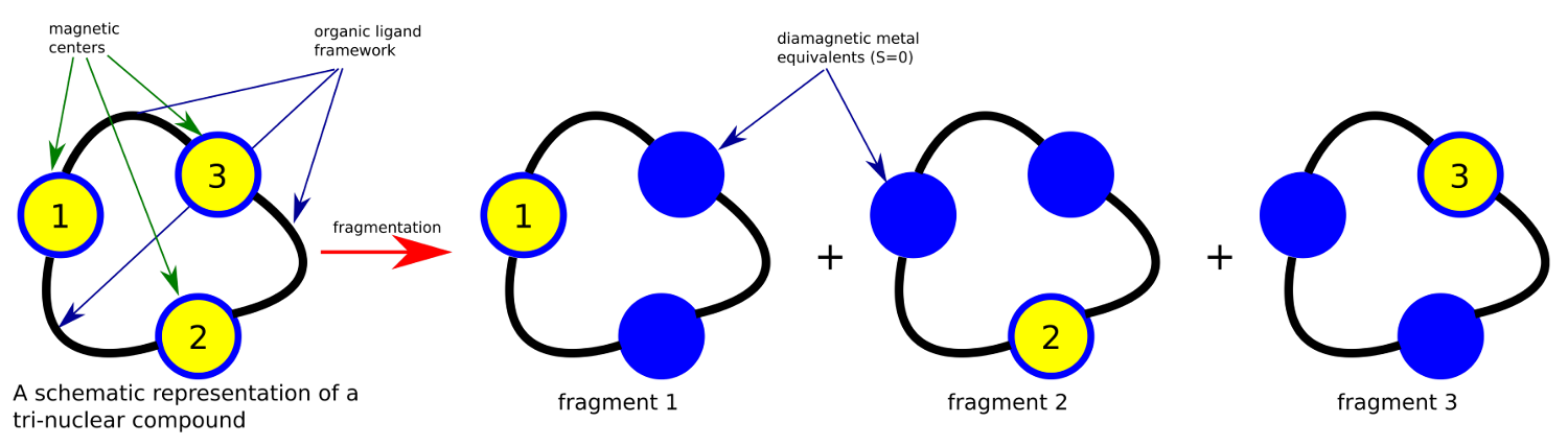
Figure 4.2.44.1 Fragmentation model of a polynuclear compound. The upper scheme shows a schematic overview of a tetranuclear compound and the resulting four mononuclear fragments obtained by diamagnetic atom substitution method. By this scheme, the neighboring magnetic centers, containing unpaired electrons are computationally replaced by their diamagnetic equivalents. As example, transition metal sites TM(II) are best replaced by either diamagnetic
Magnetic interaction between metal sites is very important for accurate description of low-lying states and their properties. It can be considered as a sum of various interaction mechanisms: magnetic exchange, dipole-dipole interaction, antisymmetric exchange, etc. In the POLY_ANISO code we have implemented several mechanisms.
The description of the magnetic exchange interaction is done within the Lines model [112]. This model is exact in three cases:
interaction between two isotropic spins (Heisenberg),
interaction between one Ising spin (only
interaction between two Ising spins.
In all other cases of interaction between magnetic sites with intermediate anisotropy, the Lines model represents an approximation. However, it was succesfully applied for a wide variety of polynuclear compounds so far.
In addition to the magnetic exchange, magnetic dipole-dipole interaction can be accounted exactly, by
using the information about each metal site already computed ab initio. In the case of
strongly anisotropic lanthanide compounds, the dipole-dipole interaction is usualy the dominant
one. Dipolar magnetic coupling is one kind of long-range interaction between magnetic moments.
For example, a system containing two magnetic dipoles
where
4.2.44.1. Files
4.2.44.1.1. Input files
The program POLY_ANISO needs the following files:
- aniso_XX.input
This is an ASCII text file generated by the Molcas/SINGLE_ANISO program. It should be provided for POLY_ANISO aniso_i.input (
- chitexp.input
set directly in the standard input (key TEXP)
- magnexp.input
set directly in the standard input (key HEXP)
4.2.44.1.2. Output files
- zeeman_energy_xxx.txt
A series of files named zeeman_energy_xxx.txt is produced in the $WorkDir only in case keyword ZEEM is employed (see below). Each file is an ASCII text formated and contains Zeeman spectra of the investigated compound for each value of the applied magnetic field.
- chit_compare.txt
A text file contining the experimental and calculated magnetic susceptibility data.
- magn_compare.txt
A text file contining the experimental and calculated powder magnetisation data.
Files chit_compare.txt and chit_compare.txt may be used in connection with a simple gnuplot script in order to plot the comparison between experimental and calculated data.
4.2.44.2. Input
This section describes the keywords used to control the standard input file. Only two keywords NNEQ, PAIR (and SYMM if the polynuclear cluster has symmetry) are mandatory for a minimal execution of the program, while the other keywords allow customization of the execution of the POLY_ANISO.
4.2.44.2.1. Mandatory keywords defining the calculation
Keywords defining the polynuclear cluster
- NNEQ
This keyword defines several important parameters of the calculation. On the first line after the keyword the program reads 2 values: 1) the number of types of different magnetic centers (NON-EQ) of the cluster and 2) a letter
TorFin the second position of the same line. The number of NON-EQ is the total number of magnetic centers of the cluster which cannot be related by point group symmetry. In the second position the answer to the question: Have all NON-EQ centers been computed ab initio? is given:Tfor True andFfor False. On the third position, the answer to the question: Are the rassi.h5 files to be read for input? is given. For the current status, the letterFis the only option. On the following line the program will read NON-EQ values specifying the number of equivalent centers of each type. On the following line the program will read NON-EQ integer numbers specifying the number of low-lying spin-orbit functions from each center forming the local exchange basis.Some examples valid for situations where all sites have been computed ab initio (case
T, True):NNEQ 2 T F 1 2 2 2
NNEQ
3  T  F
2  1  1
4  2  3
NNEQ
6  T  F
1  1  1  1  1  1
2  4  3  5  2  2
There are two kinds of magnetic centers in the cluster; both have been computed ab initio; the cluster consists of 3 magnetic centers: one center of the first kind and two centers of the second kind. From each center we take into the exchange coupling only the ground doublet. As a result the
There are three kinds of magnetic centers in the cluster; all three have been computed ab initio; the cluster consists of four magnetic centers: two centers of the first kind, one center of the second kind and one center of the third kind. From each of the centers of the first kind we take into exchange coupling four spin-orbit states, two states from the second kind and three states from the third center. As a result the
There are 6 kinds of magnetic centers in the cluster; all six have been computed ab initio; the cluster consists of 6 magnetic centers: one center of each kind. From the center of the first kind we take into exchange coupling two spin-orbit states, four states from the second center, three states from the third center, five states from the fourth center and two states from the fifth and sixth centers. As a result the
Only in cases when some centers have NOT been computed ab initio (i.e. for which no aniso_i.input file exists), the program will read an additional line consisting of NON-EQ letters (
AorB) specifying the type of each of the NON-EQ centers:A— the center is computed ab initio andB— the center is considered isotropic. On the followingnumber-of-B-centersline(s) the isotropicBare read. The spin of theBcenter(s) is defined:Some examples valid for mixed situations: the system consists of centers computed ab initio and isotropic centers (case
F, False):NNEQ 2 F F 1 2 2 2 A B 2.3
NNEQ 3 F F 2 1 1 4 2 3 A B B 2.1 2.0
NNEQ 6 T F 1 1 1 1 1 1 2 4 3 5 2 2 B B A A B A 2.12 2.43 2.00
There are two kinds of magnetic centers in the cluster; the center of the first type has been computed ab initio, while the centers of the second type are considered isotropic with
There are three kinds of magnetic centers in the cluster; the first center type has been computed ab initio, while the centers of the second and third types are considered isotropic with
There are six kinds of magnetic centers in the cluster; only three centers have been computed ab initio, while the other three centers are considered isotropic; the
There is no maximal value for NNEQ, although the calculation becomes quite heavy in case the number of exchange functions is large.
- SYMM
Specifies rotation matrices to symmetry equivalent sites. This keyword is mandatory in the case more centers of a given type are present in the calculation. This keyword is mandatory when the calculated polynuclear compound has exact crystallographic point group symmetry. In other words, when the number of equivalent centers of any kind
1followed on the next lines by as many1. Then the rotation matrices of centers of type2,3and so on, follow in the same format. When the rotation matrices contain irrational numbers (e.g.Examples:
NNEQ 2 F F 1 2 2 2 A B 2.3 SYMM 1 1.0 0.0 0.0 0.0 1.0 0.0 0.0 0.0 1.0 2 1.0 0.0 0.0 0.0 1.0 0.0 0.0 0.0 1.0 -1.0 0.0 0.0 0.0 -1.0 0.0 0.0 0.0 -1.0
NNEQ 3 F F 2 1 1 4 2 3 A B B 2.1 2.0 2.0 SYMM 1 1.0 0.0 0.0 0.0 1.0 0.0 0.0 0.0 1.0 0.0 -1.0 0.0 1.0 0.0 0.0 0.0 0.0 1.0 2 1.0 0.0 0.0 0.0 1.0 0.0 0.0 0.0 1.0 3 1.0 0.0 0.0 0.0 1.0 0.0 0.0 0.0 1.0
NNEQ
6  F  F
1  1  1  1  1  1
2  4  3  5  2  2
B  B  A  A  B  A
2.12
2.43
2.00
The cluster computed here is a trinuclear compound, with one center computed ab initio, while the other two centers, related to each other by inversion, are considered isotropic with
In this input a tetranuclear compound is defined, all centers are computed ab initio. There are two centers of type “1”, related one to each other by
In this case the computed system has no symmetry. Therefore, the SYMM keyword may be skipped.
More examples are given in the Tutorial section.
Keywords defining the magnetic exchange interactions
This section defines the keywords used to set up the interacting pairs of magnetic centers and the corresponding exchange interactions.
A few words about the numbering of the magnetic centers of the cluster in the POLY_ANISO. First all equivalent centers of the type 1 are numbered, then all equivalent centers of the type 2, etc. These labels of the magnetic centers are used further for the declaration of the magnetic coupling. The pseudo-code is:
k=0
Do i=1, number-of-non-equivalent-sites
  Do j=1, number-of-equivalent-sites-of-type(i)
     k=k+1
     site-number(i,j)=k
  End Do
End Do
- PAIR or LIN1
Specifies the Lines interaction(s) between metal pairs. One parameter per interacting pair is required.
LIN1 READ number-of-interacting-pairs Do i=1, number-of-interacting-pairs READ site-1, site-2, J End Do- ALIN or LIN3
Specifies the anisotropic interactions between metal pairs. Three parameters per interacting pair are required.
LIN3 READ number-of-interacting-pairs Do i=1, number-of-interacting-pairs READ site-1, site-2, Jxx, Jyy, Jzz End Do- LIN9
Specifies the full anisotropic interaction matrices between metal pairs. Nine parameters per interacting pair is required.
LIN9 READ number-of-interacting-pairs Do i=1, number-of-interacting-pairs READ site-1, site-2, Jxx, Jxy, Jxz, Jyx, Jyy, Jyz, Jzx, Jzy, Jzz End Do- COOR
Specifies the symmetrized coordinates of the metal sites. This keyword enables computation of dipole-dipole magnetic interaction between metal sites defined in the keywords PAIR, ALIN, LIN1, LIN3 or LIN9.
COOR
   Do i=1, number-of-non-equivalent-sites
      READ coordinates of center 1
      READ coordinates of center 2
      ...
   End Do
Other keywords
Normally POLY_ANISO runs without specifying any of the following keywords.
Argument(s) to a keyword are always supplied on the next line of the input file.
4.2.44.2.2. Optional general keywords to control the input
- MLTP
The number of molecular multiplets (i.e. groups of spin-orbital eigenstates) for which
Example:
MLTP
10
2 4 4 2 2   2 2 2 2 2
POLY_ANISO will compute the
- TINT
Specifies the temperature points for the evaluation of the magnetic susceptibility. The program will read three numbers:
Example:
TINT
0.0  330.0  331
POLY_ANISO will compute temperature dependence of the magnetic susceptibility in 331 points evenly distributed in temperature interval: 0.0 K – 330.0 K.
- HINT
Specifies the field points for the evaluation of the magnetization in a certain direction. The program will read four numbers:
Example:
HINT
0.0  20.0  201
POLY_ANISO will compute the molar magnetization in 201 points evenly distributed in field interval: 0.0 T – 20.0 T.
- TMAG
Specifies the temperature(s) at which the field-dependent magnetization is calculated. Default is one temperature point,
TMAG
6   1.8 2.0 2.4  2.8 3.2 4.5
- ENCU
This flag is used to define the cut-off energy for the lowest states for which Zeeman interaction is taken into account exactly. The contribution to the magnetization coming from states that are higher in energy than
The field-dependent magnetization is calculated at the (highest) temperature value defined in either TMAG or HEXP. Example:
ENCU
250  150
If
This means that the magnetization coming from all spin-orbit states with energy lower than
- ERAT
This flag is used to define the cut-off energy for the lowest states for which Zeeman interaction is taken into account exactly. The contribution to the molar magnetization coming from states that are higher in energy than
The field-dependent magnetization is calculated at all temperature points defined in either TMAG or HEXT. Example:
ERAT
0.75
ERAT, NCUT and ENCU are mutually exclusive.
- NCUT
This flag is used to define the number of low-lying exchange states for which Zeeman interaction is taken into account exactly. The contribution to the magnetization coming from the remaining exchange states is done by second order perturbation theory. The program will read one integer number. The field-dependent magnetization is calculated at all temperature points defined in either TMAG or HEXT. Example:
NCUT
125
In case the defined number is larger than the total number of exchange states in the calculation (
- MVEC
Defines the number of directions for which the magnetization vector will be computed. On the first line below the keyword, the number of directions should be mentioned (
MVEC
4
0.0000  0.0000   0.1000
1.5707  0.0000   2.5000
1.5707  1.5707   1.0000
0.4257  0.4187   0.0000
The above input requests computation of the magnetization vector in four directions of applied field. The actual directions on the unit sphere are:
4
0.00000  0.00000  1.00000
0.53199  0.00000  0.84675
0.53199  0.53199  0.33870
0.17475  0.17188  0.00000
- ZEEM
Defines the number of directions for which the Zeeman energy will be computed/saved/plotted. On the first line below the keyword, the number of directions should be mentioned (
MVEC
4
0.0000  0.0000   0.1000
1.5707  0.0000   2.5000
1.5707  1.5707   1.0000
0.4257  0.4187   0.0000
The above input requests computation of the magnetization vector in four directions of applied field. The actual directions on the unit sphere are:
4
0.00000  0.00000  1.00000
0.53199  0.00000  0.84675
0.53199  0.53199  0.33870
0.17475  0.17188  0.00000
- MAVE
This keyword specifies the grid density used for the computation of powder molar magnetization. The program uses Lebedev–Laikov distribution of points on the unit sphere. The program reads two integer numbers:
- TEXP
This keyword allows computation of the magnetic susceptibility
TEXP READ number-of-T-points Do i=1, number-of-T-points READ ( susceptibility(i, Temp), TEMP = 1, number-of-T-points ) End Do- HEXP
This keyword allows computation of the molar magnetization
HEXP READ number-of-T-points-for-M, all-T-points-for-M-in-K READ number-of-field-points Do i=1, number-of-field-points READ ( Magn(i, iT), iT=1, number-of-T-points-for-M ) End Do- ZJPR
This keyword specifies the value (in
- ABCC
This keyword will enable computation of magnetic and anisotropy axes in the crystallographic
ABCC
20.17   19.83   18.76    90  120.32  90
12.329  13.872  1.234
- XFIE
This keyword specifies the value (in
- PRLV
This keyword controls the print level.
2 — normal. (Default)
3 or larger (debug)
- PLOT
This keyword will generate a few plots (png or eps format) via an interface to the linux program gnuplot. The interface generates a datafile, a gnuplot script and attempts execution of the script for generation of the image. The plots are generated only if the respective function is invoked. The magnetic susceptibility, molar magnetisation and blocking barrier (UBAR) plots are generated. The files are named: XT.dat, XT.plt, XT.png, MH.dat, MH.plt, MH.png, BARRIER_TME.dat, BARRIER_ENE.dat, BARRIER.plt and BARRIER.png.
- OLDA
This keyword requests to use the old-formatted ANISOINPUT files produced by SINGLE_ANISO run. Please make use of the new DATAFILE $Project.aniso produced in any successful run of SINGLE_ANISO.